
Vibration Monitoring of Nanoscale Facilities
By
Robert E. Coleman
Senior Applications Specialist
Signalysis, Inc.
Cincinnati, OH
The Nanoscale Regime
After an ever-descending scale of microelectronics, the industry has arrived at the nanoscale. Although not yet on a massive assembly line basis, extensive R&D as well as limited production activity is taking place at the nanoscalelevel.
Figure 1 is a picture of the surface of a nanoscale specimen scanned with a resolution of approximately one nanometer (one billionth of a meter). The scan range (100 μm) is just a little more than the diameter of a human hair (80 μm). The resolution of one nanometer is only about a factor of four or five greater than the size of a carbon atom.
To gain a little appreciation for the kinds of tools employed at the nanolevel, consider some of the details of a commonly used nanoscale research tool, the Atomic Force Microscope (AFM) shown schematically in Figure 2. This marvel of ingenuity furnishes an output voltage proportional to the vertical deflection of a cantilever beam as it traverses the nanospecimen surface. The photodetector senses changes in light intensity with bending of the cantilever beam. A set of piezoelectric devices is configured to provide the translational motion (X, Y, and Z directions) of the cantilever beam, providing the raster scan. A differential voltage applied across opposite surfaces of an appropriately cleaved piezoelectric crystal will produce a small deformation (just the opposite of the action of piezoelectric crystals used in accelerometers). The raster scan, coordinated with the photodetector-generated voltage, produces a surface image on a computer screen.
This scale of operation has immediate implications for the role of mechanical vibrations. The first detail that catches one’s attention is the possibility of cantilever beam vibrations. Vibrations with deflections greater than one nanometer would certainly destroy the desired microscope resolution. Actually the intrinsic vibration characteristics of the beam itself remove it from suspicion as a problem maker: its resonance frequency may range anywhere from about 15 KHz to 300 KHz. However, resonances leading to relative vibrational motion between any of the key components within the AFM could be problematic.
Modes of Vibration
Vibration monitoring is typically performed using accelerometers with units of g as the preferred measure, so Table 1 presents some frequencies of interest with corresponding g levels (gpeak) at one nanometer (peak-to-peak displacement). Note that at any given frequency (sinusoidal motion implied) there is a simple relationship between displacement and acceleration:
![]() (1)
(1)
where X is displacement (peak), a is acceleration (peak), and Greek ν is frequency. At first glance equation 1) and Table 1 suggest it would be hopeless to control the vibration level to 50 ng at five Hz (particularly in view of the six resonance frequencies below 5 Hz associated with the vibration isolation system of Figure 2). And what about the inevitable resonances in the 300 Hz to 500 Hz range and above?
The building that a nanoscale facility may be housed in would typically be capable of participating in modes of vibration over the entire frequency range of interest. Figure 3 represents just one of about 40 or so mode shapes (deformation patterns) associated with resonance frequencies below 10 Hz (generated from a finite element model of a four story building). Similarly, the nanoscale apparatus along with associated ancillary equipment and fixturing participate in mode shapes associated with some range of resonance frequencies. Building mode shapes imply that nanoscale facilities should be located in building basements. Force generating utility equipment should be vibration isolated.
All of these considerations mean that at low frequencies, requiring something like 50 ng to 20μg control, the nanoscale apparatus must be designed so that no local apparatus flexibility modes occur in this frequency range. Base motion with displacements greater than 1 nm is acceptable as long as there is not corresponding relative motion within the nanoscale apparatus. At high frequencies, where apparatus flexibility is likely, the vibration isolation system comes into play. The isolation system is counter productive at low frequencies, generally introducing six new rigid body modes, hopefully with resonance frequencies below one to five Hz. Thus, apparatus flexibility modes should be designed for as high a resonance frequency as possible, and the vibration isolation system should be designed for maximum frequency response function roll-off above the highest of its low frequency resonances (FRF, i.e., X(ω)/F(ω)). Although more expensive, commercially available active vibration isolation closed loop control systems avoid the resonance response associated with the passive isolation systems such as that of Figure 2.
Structural Dynamic Coupling
There is a fundamental concept that should be understood about a vibrating nanoscale apparatus. The apparatus vibrates only as a participant in overall system structural modes. The kind of system we are considering is that of Figure 2, including the subground pit, seismic mass frame, apparatus housing and internal apparatus components. A given resonance frequency has associated with it a mode shape (system vibration deformation pattern) specified by mode coefficients at every point throughout the system. The coefficients are just the X, Y, Z deflections at each point for a given mode shape appropriately normalized. The mode coefficients throughout the system for every resonance frequency of interest are presented as a matrix of mode coefficients, [ Ψ ], where each column of the matrix lists coefficients (a mode shape) associated with a particular resonance frequency. The columns are known as eigenvectors; they are associated with eigenvalues, λr (λr = ωr2, r=1,2,3,…). Furthermore, the Ψ matrix performs as a transformation matrix, transforming from modal coordinates to physical coordinates:
{ X } = [ Ψ ]{ X } (2)
We press the point over the way components couple to the overall structure with the following development. The following considerations apply in general for two structures that are to be mechanically connected. Figure 5a depicts two structures that are to be coupled. We shall regard the upper structure as an operating component to be attached to a fixture (bottom structure). A grid work of measurement points has been established for each structure. Discrete degrees-of-freedom (DOF) are given for each point, i.e., x, y, z displacement coordinates. Displacements for all DOF (coordinates) of a given structure can be represented by a column vector, { X }.
Let’s assume a modal analysis has been performed on the operating component and its DOF may be represented in modal coordinates by the column vector, X
C . DOF of the fixture are partitioned into two groups, XA and XB. XB represents those degrees-of-freedom that are to be connected to the upper operating component. The uncoupled dynamical equations of motion for both structures, the operating component and fixture, before connection may be written in matrix form:
![]() (3)
(3)
where the dynamical matrix has been partitioned into the diagonal modal dynamical matrix, DCC , of the operating component and the submatrices of the fixture dynamical matrix, D (further partitioned into DAA, DAB, DBA, and DBB). The right side of the equation is a column vector of forces, partitioned into the appropriate coordinates (DOF), representing any arbitrary forces that might be applied to the two structures.
After connecting the two structures (Figure 5b), physical degrees of freedom, XB, of the fixture are constrained to participate in the modal deformations corresponding to the modal coordinates, XC. Notice that no matter what deformations result at the common interface points, those deformations can always be decomposed into superpositions of the XC mode shape deformations along the interface. This may be expressed mathematically as the coordinate transformation from modal coordinates to the XB physical coordinates:
![]() (4)
(4)
Thus, the two structures are coupled into a global system through the constraint equations,
 (5)
(5)
Substituting equation 5) into the equation 3) system equation and premultiplying both sides by the transposed coupling matrix of equation 5), we have the coupled system equations,
Carrying out the indicated matrix operations yields
![]() (7)
(7)
Now, with the development of equation 7), the global character of the new combined structure is appreciated. There is manifestly one total structure now, even though one can recognize the participation of the individual components. In fact new global system resonance frequencies and mode shapes can be found by solving a new eigenvalue-eigenvector problem. Indeed, the new system dynamical matrix may be diagonalized using the new system mode shapes, [ Φ ], to yield a new dynamical matrix, given in a new set of modal coordinates, DDD:
![]() (8)
(8)
So, we have the new coupled system equations in the new modal coordinates,
![]() (9)
(9)
One of the implications here is that you may not correctly anticipate the apparatus resonance frequencies as reported by a vendor. We have system resonances that depend on the final coupled system rather than just apparatus single component modes. In fact the vibration response, { XD }, of points on the system due to forces, { FD }, applied at points on the system may be expressed using a superposition of the newly coupled system modal FRFs (the matrix of FRFs, [ H(ω) ], is the inverse of the dynamical matrix, [D(ω)]). For a pair of points, j (measured response displacement DOF) and k (applied force DOF), the FRF, hjk(ω)=Xj(ω)/Fk(ω), i.e., ratio of Fourier Transforms of displacement and force, is
where βr is the frequency ratio, ω/ωr, for the rth mode, ζr is the damping fraction (ζ = c/cc, i.e., viscous damping constant over critical damping) for the rth mode, and mr is modal mass for the rth mode.
Vibration Monitoring System Requirements
A monitoring system may include measurements of static displacements, angular motion, vibration displacement, velocity and acceleration on floor, wall, seismic mass, equipment frame and nanoscale apparatus. Here we focus on acceleration and velocity spectra.
The monitoring system should include sensitive accelerometers, a computer with appropriate data acquisition capability and robust software. The National Instruments data acquisition board, NI4472B, is particularly well suited. Its bit resolution, analog dynamic range, low frequency range, available sampling rates, anti-aliasing, parallel sample and hold, and built-in signal conditioning for ICP accelerometers make it a good match for nanoscale monitoring requirements.
The application software should provide a wide variety of data displays, including time histories, 1/1 and 1/3-Octave spectra and narrow band spectra. Simultaneous display of short and long averaged narrow band spectra is useful. Also, simultaneous displays of fine resolution (~0.1 Hz) and course resolution (~2 Hz) are often required. Spectrum plots should have a range of normalization selection, such as RMS, peak, amplitude, amplitude per sqrt(Hz), and PSD along with user control over units. Continuous long-term monitoring with time domain and frequency domain trending is required. A particularly critical component of the monitoring process is the automatic generation of reports. Database management must accommodate the extremely large accumulation of data and allow quick access to historic data. Database filtering methods are essential.
Simulated Monitoring Example
An example of facility monitoring is presented here using a scaled down simulation. Figures 6 and 7 show a test setup used to simulate conditions of a seismic mass vibration isolation system installed on a building upper floor (aluminum table). The isolation system consists of two 27 lb steel weights mounted on lead-lined foam cushions. A PCB seismic accelerometer with sensitivity of 10 V/g is at 4Z, and accelerometers at 1Z, 2Z and 3X have sensitivities of 100 mV/g.
Figure 8 shows a screen display for data acquired during a quiet floor environment. A legend for the identification of the displays is shown in Figure 9. Figure 10 is a plot of the accelerometer 4Z acceleration spectral density (ASD) vs. frequency (logASD vs. linear frequency). ASD has units of grms/sqrt(Hz). It is simply the square root of the power spectral density (PSD). All narrow band spectral data have been normalized in this fashion to allow comparisons among spectra having different spectral resolution.
The lower curve of Figure 10 represents the National Instruments open circuit input noise floor. Note that the quiet floor vibration level is well above the noise floor. Once connected, the accelerometer and cable contribute a small additional component of electrical noise, particularly at 120 Hz. ASD facilitates easy upper bound estimates of RMS levels over a selected frequency range. For example it is seen that summing up the ASD-squared values from 100 Hz to 500 Hz, then taking the square root, the grms value over that range is certainly less than 4 μgrms. This is considerably less than the 20 μg level corresponding one nanometer at 100 Hz from Table 1 (note 180 μg at 300 Hz, etc.).
The seismic mass 4Z 1/3-Octave velocity spectrum is plotted in Figure 11 as log(Vrms) vs. log(frequency). Here we have included an upper alarm level corresponding to a modified NIST-A1 vibration monitoring specification3 (the lower curve references the electronics noise floor). If a specification limit is violated, the monitoring system will set off audible alarms as well as flash a red border around the corresponding screen display. Additionally, a telephone call will be automatically placed to selected phones to provide personal alerts. Specifications for various classes of facilities are given in Table 2. Our seismic mass is seen to be considerably under the alarm level and comfortably above the electronics noise floor.
The 100 mV/g accelerometers (1Z, 2Z and 3X) make a poor choice for nanofacility monitoring as is seen in the plot of Figure 12 for accelerometer 1Z. The data for a quiet floor barely rise above the noise floor.
Other Monitoring Metrics
Another method of processing considered here to be of potential benefit to facility monitoring is the Shock Response Spectrum (SRS)5. It is felt that current specifications do not properly account for transient events. The SRS is a natural metric for representing the severity of transient events, because it anticipates the internal peak displacement response for each possible mode of vibration for an apparatus mounted on a seismic mass. However, this would not be expected to be a real-time continuous monitoring process.
Yet another method that could prove fruitful would be one using an FRF (frequency domain). Assume that, while applying a vibratory force to the base structure, an FRF function is obtained between the base structure and the voltage output (proportional to displacement) of an AFM. The AFM is maintained in a fixed position. The FRF might have the form, h(ω) = X(ω)/g(ω), where X(ω) is the Fourier Transform of the relative displacement motion within the AFM and g(ω) is the Fourier Transform of the base acceleration. Now, as a part of vibration monitoring during normal operation of the AFM, base acceleration Fourier Transforms may be computed continuously, and continuous estimates of AFM relative displacement spectra could be displayed using the product of the FRF and the Fourier Transform of acceleration, i.e., X(ω) = h(ω)g(ω). Further, the Inverse Fourier Transform could be performed on the resulting X(ω), should the displacement time history be desired. Appropriate alarm limits might be established.
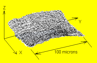
Figure 1. Image of surface from a nanoprobe scan with resolution of approximately one nanometer.
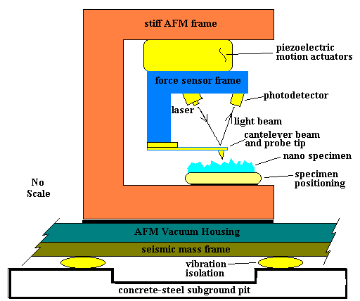
Figure 2. Schematic of an Atomic Force Microscope. One possible scheme for mounting the microscope for vibration isolation is indicated. The concrete-steel subground pit rests on solid earth about ten to fifteen feet below ground level. The pit should be free of contact with the laboratory ground level floor.
| Frequency Hz | g level at 1 nm |
| 5 | 50 ng |
| 10 | 201 ng |
| 30 | 1.8 μg |
| 100 | 20 μg |
| 300 | 180 μg |
| 500 | .5 mg |
Table 1. G levels corresponding to a displacement of one nanometer (1 nm) for selected frequencies.
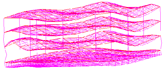
Figure 4. Four story building mode shape from finite element model. Resonance frequency: 9.69 Hz. Mode number: 46.
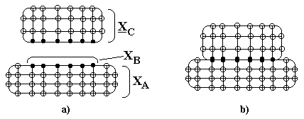
Figure 5. Attaching an operating structural component to a base structure (test fixture). The component is described using its modal coordinates, XC, and the fixture is described using physical coordinates (numbered DOF on the structure). The physical coordinates of the fixture are divided into XA and XB (points to be connected).
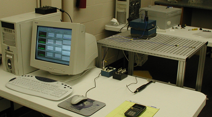
Figure 6. Test setup for facility seismic mass vibration isolation system simulation.
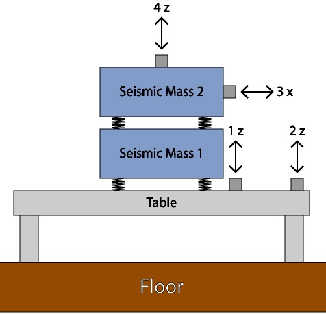
Figure 7. Simulated nanofacility vibration isolation system for vibration monitoring exercise. Four accelerometers are installed. Two steel blocks, 27 lb each, are mounted on lead-lined rubber cushions.
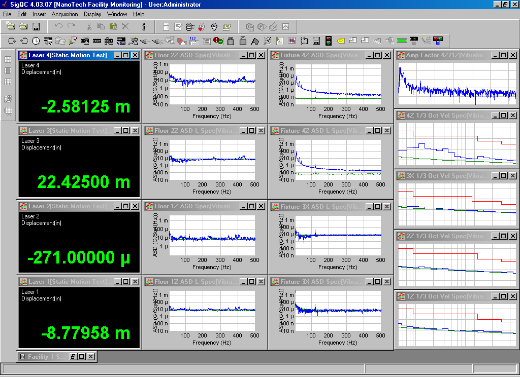
Figure 8. Screen display for data acquired for a quiet floor vibration environment. Digital displays are laser displacements and other windows are vibration spectra.
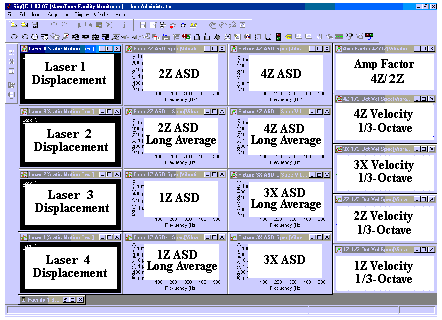
Figure 9. Legend identifying data displays of Figure 8.
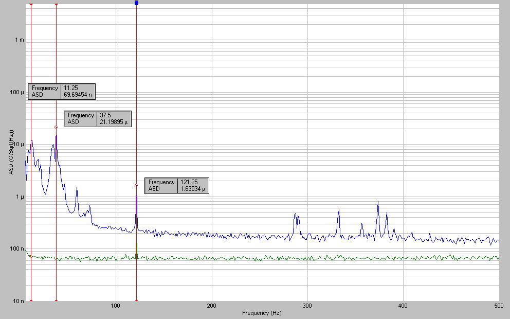
Figure 10. Narrow band ASD of seismic mass quiet floor vibration acquired from accelerometer 4Z. The lower curve is a measure of the electronics noise floor.
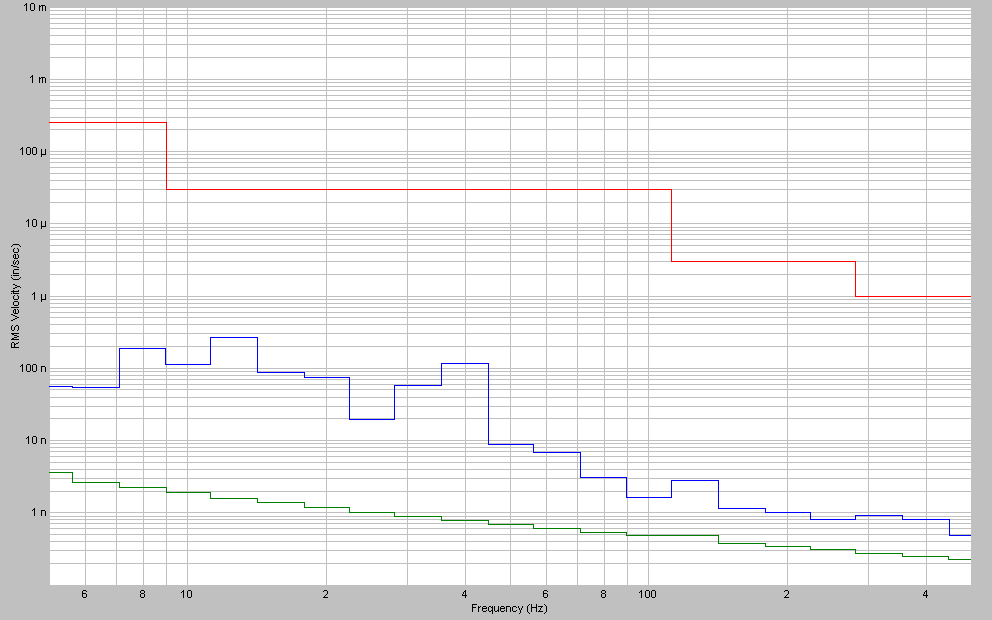
Figure 11. 1/3-Octave velocity (in/sec rms) spectrum from the 4Z seismic mass quiet floor vibration measurement –log(Vrms) vs. log(frequency). The vibration level is well above the electronics noise floor (lower curve) and well below the NIST-A1 alarm level.
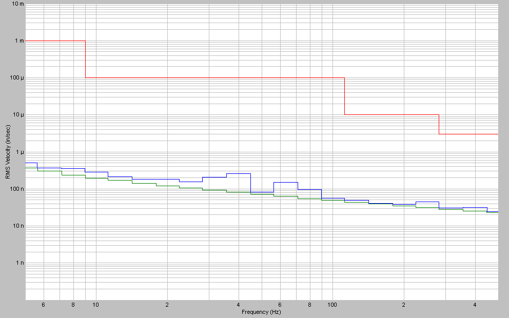
Figure 12. 1/3-Octave velocity (in/sec rms) spectrum from the 1Z floor accelerometer for the quiet floor vibration measurement –log(Vrms) vs. log(frequency). The vibration level in this case is barely above the electronics noise floor (lower curve), but well below the NIST-A1 alarm level.
| Category | Criterion | Definition (μin/s) |
| Human Sensitivity | ISO Office | 16K – 32K |
| Generic Laboratory | VC-A | 2000 |
| “ | VC-B | 1000 |
| Highly Sensitive | VC-D | 250 |
| “ | VC-E | 125 |
| “ | NIST-A | 1 μin displacement (1-20Hz)
125 μin/s (20 – 100Hz) |
| Ultra Sensitive | NIST-A1 | 250 (1-5Hz)
30 (5-100Hz) |
Table 2. Specifications for upper limits on vibration levels for different facility categories. A modified NIST-A1 was used for examples in this paper. (See ref. 3)
References
- Structural Dynamics
An Introduction to Computer Methods
Roy R. Craig, Jr.
Dept. of Aerospace Engineering & Engineering Mechanics
The University of Texas at Austin
John Wiley & Sons, N.Y.
- Experimental Structural Dynamics
An Introduction to Experimental Methods of Characterizing Structures
Robert E. Coleman
Senior Applications Specialist
Signalysis, Inc., Cincinnati, OH
AuthorHouse
Bloomington, IN
- Facility Vibration Issues for Nanotechnology Research
Hal Amick, Michael Gendreau and Colin G. Gordon
Colin Gordon & Associates, San Bruno, CA, USA
Nano Devices Technology 2002
May 2-3, 2002, National Chiao-Tung University, Hsinchu, Taiwan
- Vibration Design of 300mm Wafer Fabs
Tao Xu, Hal Amick and Michael Gendreau
Colin Gordon & Associates, San Bruno, CA USA
tao.xu@colingordon.com
- SRS article on Signalysis website: signalysis.com