

by Robert E. Coleman
Signalysis, Inc.
Cincinnati, OH
A discussion of vibration theory usually begins with the analysis of a simple mass, spring and damper system. This is because once you analyze the vibration process for this system you can then apply the results to the most complicated vibrating structure. It will be shown later how complex structures vibrate in a superposition of a unique set of different deformation patterns (called mode shapes). Each mode shape has its own resonance frequency and responds to vibratory forces in a manner described by the same differential equations as are used to describe single mass, spring and damper vibration response.
Figure 3 represents a mass, m1, supported by a spring of stiffness, k1, and a damper having a viscous damping value, c1. Consider a vibratory force, f1, applied to the mass as indicated in the free body diagram. The spring and damper react with forces, fk and fc, and the algebraic expressions for these forces are given as Hook’s Law for the spring and the viscous force formula for the damper. The motion resulting from the applied force and reaction forces is given by Newton’s Second Law as shown in the figure.
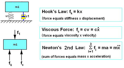
Figure 3. Vibration motion of a mass supported by a spring and a damper and responding to an applied vibratory force is analyzed using Newton’s Second Law.
Expanding the Newton’s Law equation of Figure 1 and rearranging gives
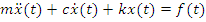
(1)
Since we are interested in the way the system vibrates at the various frequencies across the spectrum it is convenient to perform the Fourier Transform on equation 1), expressing all variables as a function of frequency, ω (radians/sec), rather than time.

(2)
Note that frequency in Hz, ν, is equal to (1/2π)ω.
This second order differential equation with constant coefficients may be expressed as an algebraic equation if we take note that at any frequency of the spectrum there are simple algebraic relationships between displacement, velocity and acceleration:
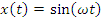
(3)

(4)
where we have used the imaginary number, I, to represent the 90-degree phase shift between the cosine and sine functions.
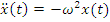
(5)
Since these equations apply at all frequencies across the spectrum we see that they provide us with the Fourier Transforms so that equation 2) may now be written as an algebraic equation (no derivatives) using displacements in place of velocity and acceleration.

(6)
Now we can factor out the displacement:

(7)
At this point we will not focus on the displacement solution of the equation, but rather we wish to find the ratio, displacement divided by force. This is known as the Frequency Response Function (FRF), h(ω):
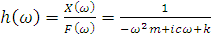
(8)
The FRF may be presented in a more useful form after rationalizing the denominator and introducing a couple of new definitions for β and ζ.
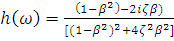
(9)
β = ω/ωr (ratio of frequency to resonance frequency)
ζ = c/cc (ratio of damping to critical damping)
With a damping value, c, equal to zero the mass-spring-damping system, if released from a displaced position, would vibrate indefinitely. The damping is said to be underdamped if, when released from a displaced position, the mass-spring-damping system vibrates at resonance but decays with time. if the damping value has a value known as the critically damped value, cc, there will be barely enough damping to avoid oscillation.
Consider the process in which the system of Figure 3 is excited into free vibration using an impact force applied with a hammer. The impact force (during the brief time the hammer is in contact with the mass) has the form of a half-sine pulse that is very short compared to one cycle of vibration.
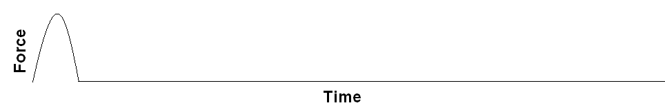
Figure 4. The force-time pulse resulting from a hammer impact applied to the mass of Figure 3.
At a time very close to zero time (force pulse has terminated), the displacement of the mass is approximately zero, the velocity has some value, v0, and the acceleration is zero. Now, the system vibrates at its resonance frequency, decaying in accordance with the solution of the differential equation 1):

10)
Where V0 is the initial velocity, ν is the system resonance frequency, and ζ is the damping factor. This solution is graphed in Figure 4.
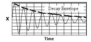
Figure 5. Damped oscillations from solution to the mass-spring-damper system differential equation. The dashed curve envelopes the positive peaks.
Now, getting back to the frequency domain solution of equation 9), we will consider this solution from a different point of view. Having derived the FRF from the differential equation, we now consider the way in which we may develop the FRF experimentally. Consider now that we have acquired the force vs. time of Figure 4 by measuring the force. The hammer used for the impact force includes a force transducer in the hammer tip and the force-time signal is captured into our computer. A Fourier Transform is performed on that data yielding a force vs. frequency spectrum, F(ω). Simultaneous with capturing the force signal, we also capture the decayed displacement vs. time data represented by Figure 5 and perform the Fourier Transform on this data as well. Forming the ratio of these two Fourier Transforms, X(ω)/F(ω), returns data having exactly the same functional form as our FRF of equation 9).
The magnitude of the FRF is plotted versus frequency as Figure 6. Notice, as would be expected, the peak in the curve occurs at the resonance frequency.
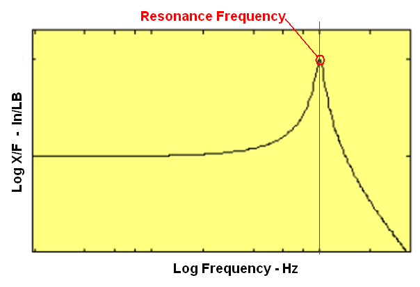
Figure 6. FRF computed from measurements of force and displacement vibration on the mass of Figure 3. The FRF is formed from the ratio of the Fourier Transform of displacement divided by the Fourier Transform of Force.
Remember that the FRF equation 9) includes a Real Part and an Imaginary Part. These two functions are plotted as Figure 7. A significant feature of these two functions is that the Imaginary Part peaks negatively (negative valley) at the resonance frequency and the Real Part crosses zero at resonance.
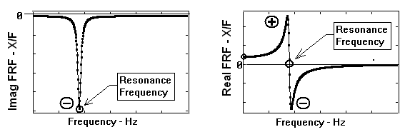
Figure 7. Plots for the FRF Imaginary Part (left) and Real Part (right).
Now, consider the characteristics of a general vibrating structure having many masses and springs or extended materials combined in arbitrary configurations. The structure could be entirely cast, made of welded pieces or assembled with bolted joints. It can be shown that the Imaginary Part measured at various locations on a structure such as these may be used to see the mode shape associated with a given resonance frequency. When vibrating under the influence of a vibratory force, there is a phase angle between the displacement and the force for any given frequency in the spectrum. At resonance the phase angle between the displacement and applied force is either +90-degrees or -90-degrees. The imaginary number, either +I or -I, of course represents a plus or minus 90-degree phase shift.
Figure 8 illustrates the concept of multiple resonance frequencies and mode shapes. Here sketch the deformation patterns (mode shapes) of a cantilever beam, each of which is associated with different resonance frequency. If you were somehow able to deform the cantilever beam in one particular mode shape, then release it, the beam would vibrate naturally with the resonance frequency.
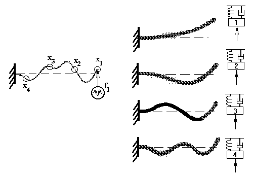
Figure 8. The first four mode shapes of a cantilever beam. Each mode shape behaves as a single mass-spring-damper system. The beam can freely vibrate in any one of the modes at the resonance frequency associated with that mode.
When an FRF measurement is performed on a multi-degree of freedoms system such as the cantilever beam, a hammer impact will excite all modes simultaneously. Each mode behaves just like a single mass-spring-damper and has its own FRF that looks just like the FRF of Figure 6. The result for the measured FRF is a linear superposition of all modal FRFs. Accordingly, the actual deformation at a given instant during vibration might look like that on the left side of the Figure 8 sketch. There we see that the unique mode shapes of the structure all vibrating individually (behaving like individual single mass-spring-damper systems), yet they all sum together to produce the measured deformation.
Figure 9 emphasizes the sense in which each mode shape behaves just like a single mass-spring-damper. The single mode FRF’s are shown with each corresponding mode shape with its single mass-spring-damper model.
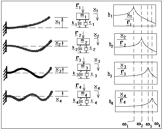
Figure 9. A single mass-spring-damper modal FRF is associated with each individual mode shape of the cantilever beam.
We think of each mode shape as having a modal mass, modal spring and modal damper. The collection of forces across the beam required to force just one mode shape may be represented as a single modal force. A modal displacement value may be derived that represents the modal deformation amplitude with a single modal displacement value.
An FRF measured on a structure may be analyzed as a superposition of the individual modal FRFs as suggested in Figure 10. Three modal FRFs are summed together to give the total FRF (heavy curve) that would be measured experimentally. The plus and minus symbols indicate a positive or negative phase over a given frequency range. Modal FRFs cancel in a region where they are in opposite phase. Mode coefficients shown with the Greed psi symbols provide the weighting for each modal FRF in the summation. Further discussion of these details is beyond the scope of this discussion.
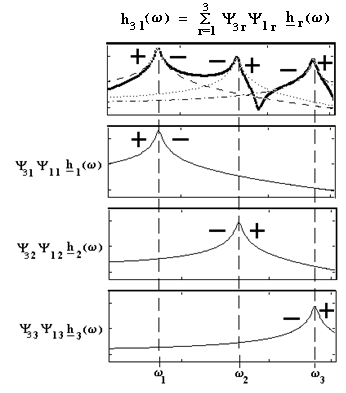
Figure 10. The superposition of three modal FRFs. The positive and negative symbols indicate the phase relationship between response motions for the given modes as compared to the force as reference.
The NASA Space Shuttle is used below (Figure 11) to illustrate mode shapes for a fairly complex structure. During the ascent phase of one shuttle mission high speed movies using a special high resolution telescopic lens capture unexpected violent vibration of an Orbiter subsystem known as the Body Flap. Later, experimental modal analysis was performed on the Body Flap to identify its resonance frequencies and mode shapes and to use this information as part of an effort to estimate the fatigue life of the structure.
The first three mode shapes of the Body Flap are shown in Figures 12, 13, and 14. These modes were analyzed both experimentally as well as mathematically using the Finite Element Method (FEM).
These tools could be applied to the analysis of aluminum castings. However, a careful review of the applicability to the particular end goal should be assessed before committing to a particular method.
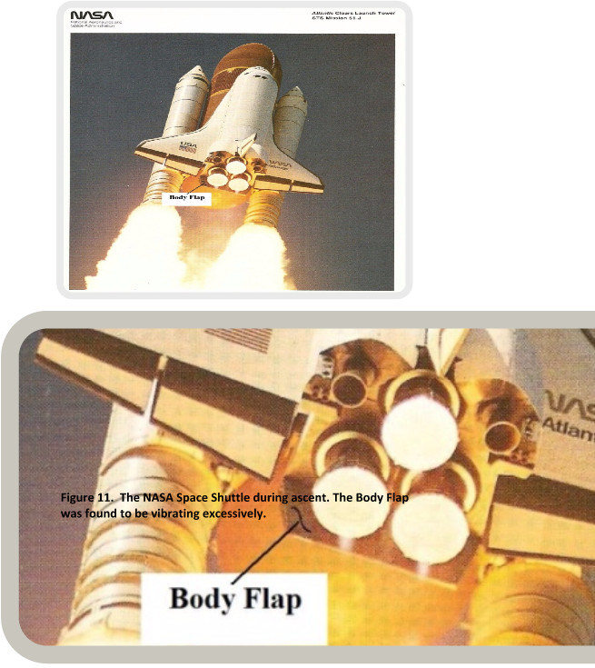
Figure 11. The NASA Space Shuttle during ascent. The Body Flap was found to be vibrating excessively.
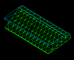
Figure 12. Body Flap mode shape 1. Rotation about the Aft Fuselage Actuator attachment system. Resonance frequency during flight: 8Hz. Original resonance frequency before any flights: 12Hz.
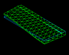
Figure 13. Body Flap mode shape 2. First torsion mode. Resonance frequency: 14Hz.
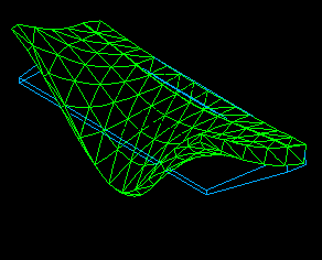
Figure 14. Body Flap mode shape 3. Two-node bending along trailing edge.